2: Word Embeddings
A large proportion of the efforts of the research and commercial community in NLP has been focused on processing the data in the best way possible for downstream applications. The methods that we have covered so far has been the result of a continuous evolution in preserving information for machine learning inference. One of the largest breakthroughs in NLP has been the invention of word embeddings.
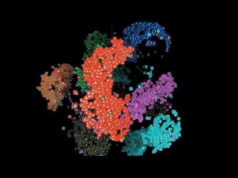
The basic assumption about word embeddings is that every single word is defined largely by its context. That is words that mean roughly the same thing, appear in similar contexts. Thus if you take a sufficiently large (and diverse) dataset, it is possible to define each word based on its distance from the others. You can imagine a giant cloud where each individual word is a droplet, and is surrounded by similar words, where the distance is this similarity (in this context a cosine distance is used). How it works is visualised on Visualsiation of word2vec. Note how if we color the vectors based on their values, similar vectors (like “king” and “queen”) will have similarities, while something like “water” would be very different..
Word Embeddings | Rasa (7 minutes)

In the end of the embeddings process every word is represented by a n-dimentional vector (i.e. “coordinates” in the the cloud), that can be used as an imput to a machine learning model. With some linear algebra we can replace spam and ham SMS messages with their respective embeddings, and feed that to a machine learning classifier, such as as Random Forest (even though deep learning methods are often much more accurate in this context).
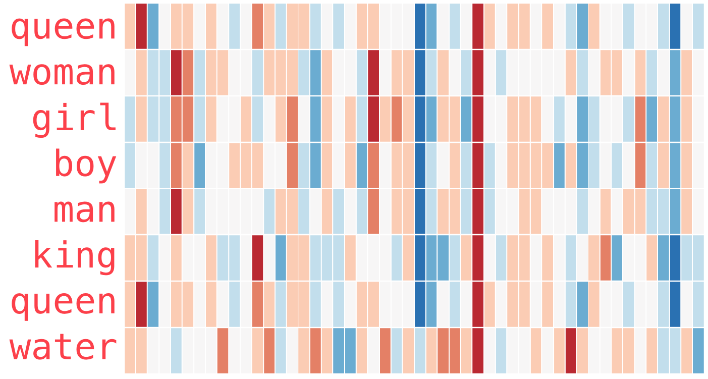
Fig. 3 Visualsiation of word2vec. Note how if we color the vectors based on their values, similar vectors (like “king” and “queen”) will have similarities, while something like “water” would be very different.
For some domain specific use cases (let’s say you have a very specific dataset, such as in the medical domain, that contains a lot of abbreviations that are specific to that case and are not normally encountered in other corpora) it makes sense to create our owm word embeddings. But for most NLP applications it makes sense to take advantage of pre-trained models, for example those computed on Wikipedia or other similar datasets, that are available for free.
Blended learning: TensorfFlow Word2vec
TensorFlow is one of the two most popular deep learning open source libraries, supported by a few companies, and originating at Google. They have also provided an excellent tutorial on how to use Tensorflow to create your own embeddings. We will be covering how to do this in this module, but if you want to have a deeper understanding it is useful to have a look at that tutorial, available here (45 minutes).
Blended learning: Illustrated Word2vec
A lot of the topics covered in data science can be a bit abstract to grasp at first, and some might have an easier way to do that with visual understanding. Have a look at an excellent illustrated and detailed guide to word embeddings with word2vec here (1 hour).
Making custom word embeddings with Fasttext

Fasttext is an open-source NLP library from Facebook. Since it is a product of a large company which deals with huge quantities of text data, this software is built for performance, usability and scale.
While Fasttext contains also modules for other NLP tasks, such as classification and language detection, for the purposes of this tutorial we will focus on creating custom word embeddings.
We will also use another open source library, called gensim to use those word embeddings. This is a library that can also be used for other NLP tasks, such as unsupervised learning (i.e. Topic Modeling), but that will be covered in a separate section.
Blended learning: Fasttext paper
In order to gain complete understanding it makes sense to invest time in reading the fundamental original work (there are a multitude of papers on the topic, but just a few of them are very influential and inspire the further research).
The original Fasttext research paper from Facebook is one such paper, and you can read it here (1 hour).
import fasttext
import pandas as pd
from gensim.models import FastText as fText
from gensim.models.fasttext import load_facebook_vectors
As a first step for training our embeddings we should store the original .csv in a format that is suitable for fasttext. This format is a plain .txt file, with one column containing the text (one entry per line), and also no headings or index.
Stanford CS224N: NLP with Deep Learning | Winter 2019 | Lecture 1 – Introduction and Word Vectors (1.5 hours)
Stanford CS224N: NLP with Deep Learning | Winter 2019 | Lecture 2 – Word Vectors and Word Senses (1 hour)
reviews_data = pd.read_csv("../data/reviews_data.csv")
reviews_data["reviewText"].to_csv("../data/reviews_data_embeddings_training_data.txt", header=False, index=False, sep="\t", mode="a")
Now that we have the data prepared, we can start to train the model. For this we use the train_unsupervised function.
model = fasttext.train_unsupervised("../data/reviews_data_embeddings_training_data.txt", model="skipgram")
Now that we have the model we should store it for a future use.
model.save_model("models/reviews_vec.vec")
There are different options that can be used to load those embeddings, but for our use case we will use the gensim pacakge.
fastText_wv = load_facebook_vectors("models/reviews_vec.vec")
Now let’s have a look what can we actually do with those embeddings, and do they make sense? One thing which we can try is to compute the most similar to a specific word embeddings, let’s see payment:
fastText_wv.most_similar("service")
[('guy', 0.9153076410293579),
 ('visit', 0.9117871522903442),
 ('$75', 0.8935893177986145),
 ('paying', 0.8484381437301636),
 ('Weve', 0.8340294361114502),
 ('4-5', 0.8236839771270752),
 ('months', 0.7747606635093689),
 ('per', 0.7211363315582275),
 ('routed', 0.6958457231521606),
 ('appliance', 0.6802433729171753)]
Those are sorted by cosine similarity. How does an individual word look like?

Fig. 4 Cosine similarity
Blended learning: Cosine similarity
Read more about cosine similarity and the math behind it here (1 hour).
Exercise
Imagine your task is to build a tool that sorts job candidates based on their similarity. How could you approach this problem with custom word embeddings? Write up a pseudo-code description of your approach.
fastText_wv["service"]
array([ 0.03369893, -0.30342257, -0.31287557,  0.06328347, -0.15422097,
        0.6900311 ,  0.2902713 , -0.04522721,  0.12707095, -0.10173076,
       -0.35954508, -0.37574846,  0.3420938 , -0.14806445, -0.06105737,
       -0.6152239 ,  0.48375046,  0.31523395, -0.41773838, -0.25677437,
        0.39742705, -0.00882626,  0.24042241,  0.60639435, -0.6874998 ,
        0.20789383,  0.5564708 , -0.48442906,  0.19938357, -0.42489457,
       -0.25001803,  0.12958974, -0.5063852 ,  0.17509942, -1.0968775 ,
       -0.57158804, -0.36259872, -0.23189294, -0.19346552,  0.5832819 ,
        0.18999015, -0.06430916,  0.7494559 , -0.56587875,  0.3883682 ,
        0.6603875 ,  0.4528623 , -0.6583048 ,  0.18912114,  0.07246456,
       -0.1075282 ,  0.09732103, -0.32490987,  0.68329686, -0.12884144,
        0.17648453, -0.48592442, -0.1735929 , -0.40970507,  0.40856415,
       -0.49658212, -0.58721876,  0.01796373,  0.6114106 , -0.43736   ,
       -0.50215924,  0.786839  ,  0.77078503,  0.09432894, -0.40565056,
       -0.80805415,  0.42209527, -0.24033622, -0.50208396, -0.7655079 ,
       -0.56293756, -0.25264573, -0.6587055 , -0.39461687, -0.3533211 ,
        0.17465983, -1.3165748 , -0.05236346, -1.1126766 , -0.01922854,
       -0.40551388, -0.03952708,  0.77595365,  0.1453283 ,  0.34026647,
        1.0555615 , -0.71291816,  0.7598502 ,  0.4585296 , -0.720232  ,
        0.0925275 , -0.6108507 ,  0.2989141 , -0.51312596,  0.31303704],
      dtype=float32)
Additional information
By using any pre-trained model, we are relying on the assumption that the data it was trained upon is representative. Of course, this is not always the case, and word embeddings are no exception. In order to get some context on how bias can creep in this technology as well, read this blog post from Google Developers explaining the issue.
As we imagined, this is a vector of length 300.
Word Embeddings Visualisation with t-SNE
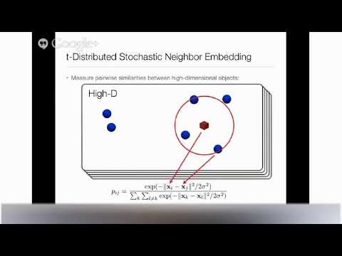
So we can keep manually investigating if those embeddings make sense, but is there a better way? One thing we can do to have a higher level overview on the quality of our embeddings, and perhaps even to find some hidden patterns is to try to visualise these vectors. This is not a simple task, since the vectors are n-dimentional (in our case 100), and visualising this on a 2-D or 3-D plane, which is understandable for humans, while preserving roughy the relationships requires a special algorithm.
One option is called t-SNE, which is accessible from the scikit-learn package. Let’s give it a try.

from sklearn.manifold import TSNE
import matplotlib.pyplot as plt
# set figure sizes for plots
from pylab import rcParams
rcParams['figure.figsize'] = 20, 20
X = fastText_wv.wv[fastText_wv.wv.vocab]
/Users/boyanangelov/misk/misk-nlp/venv/lib/python3.6/site-packages/ipykernel_launcher.py:1: DeprecationWarning: Call to deprecated `wv` (Attribute will be removed in 4.0.0, use self instead).
  """Entry point for launching an IPython kernel.
Exercise
t-SNE is not the only method that can be used for visualising highly dimentional data. Can you find and describe another one?
tsne = TSNE(n_components=2)
X_tsne = tsne.fit_transform(X)
The code below will plot the results in 2-D, while also annotating 300 words (we could annotate more, of course, but the readability of the plot might suffer from too much text).
Vizualizing Data Using t-SNE (Google Tech talks) (1 hour)
plt.scatter(X_tsne[:, 0], X_tsne[:, 1])
words = list(fastText_wv.wv.vocab)[0:300]
for i, word in enumerate(words):
	plt.annotate(word, xy=(X_tsne[i, 0], X_tsne[i, 1]))
plt.show()
/Users/boyanangelov/misk/misk-nlp/venv/lib/python3.6/site-packages/ipykernel_launcher.py:2: DeprecationWarning: Call to deprecated `wv` (Attribute will be removed in 4.0.0, use self instead).

Now we can see that there are some clusters of words that are starting to form, and hopefully those make sense.
A.I. Experiments: Visualizing High-Dimensional Space (3 minutes)
Using pre-trained word embeddings
Beyond word2vec: GloVe, fastText, StarSpace (40 minutes)
Now that we have learned how to use our own word embeddings, let’s learn how to use pre-trained ones. As a first step we should download them. A good set is available here, and to download use this command
wget http://nlp.stanford.edu/data/glove.6B.zip
Depending on the speed of your internet it might take a while. Let’s first load the packages we need:
GloVe - Python for Word Representation (30 minutes)

from tqdm import tqdm
import numpy as np
import pandas as pd
from nltk.corpus import stopwords
from nltk import word_tokenize
from sklearn.preprocessing import LabelEncoder, StandardScaler
from sklearn.model_selection import train_test_split
from keras.utils import np_utils
import pickle
Using TensorFlow backend.
stop_words = set(stopwords.words('english'))
le = LabelEncoder()

X = reviews_data["reviewText"]
y = reviews_data["overall"]

X_train, X_test, y_train, y_test = train_test_split(
    X, y, test_size=0.33, random_state=42)
This is where we load the embeddings from the raw file into a dictionary.
embeddings_index = {}
f = open('../data/glove.6B.300d.txt')
for line in tqdm(f):
    values = line.split()
    word = values[0]
    coefs = np.asarray(values[1:], dtype='float32')
    embeddings_index[word] = coefs
f.close()
400000it [00:35, 11264.77it/s]
Blended learning: GloVe
Read the GloVe paper (1 hour)
The following function does some processind and algebra to convert a piece of text into a 300 dimentional vector. Credit for this function goes to Abhishek Thakur (see Blended learning below).
Additional information: How to Approach Any ML Problem on Kaggle
![]()
Abhishek has a great tutorial, called “Approaching (Almost) any NLP Problem on Kaggle”. It provides a useful summary of a lot of the things we have learned so far, so it would be useful for you to go through. You can find it as a Kaggle Kernel here.
Approaching (almost) Any Machine Learning Problem | by Abhishek Thakur | Kaggle Days Dubai (45 minutes)

def sent2vec(s):
    words = word_tokenize(s)
    words = [w for w in words if not w in stop_words]
    words = [w for w in words if w.isalpha()]
    M = []
    for w in words:
        try:
            M.append(embeddings_index[w])
        except:
            continue
    M = np.array(M)
    v = M.sum(axis=0)
    if type(v) != np.ndarray:
        return np.zeros(300)
    return v / np.sqrt((v ** 2).sum())
And finally we can use this function to replace the words of our data with embeddings:
X_train_glove = [sent2vec(x) for x in tqdm(X_train)]
X_test_glove = [sent2vec(x) for x in tqdm(X_test)]
100%|██████████| 1525/1525 [00:04<00:00, 306.51it/s]
100%|██████████| 752/752 [00:02<00:00, 308.10it/s]
Next there are a few additional transformations that we need to do before we are done with preparing the data for machine learning. The most important one of those it to scale the data. The difference between scaling and standardisation is shown on Scaling and Normalization.
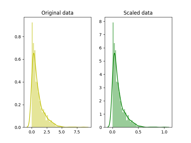
Fig. 5 Scaling
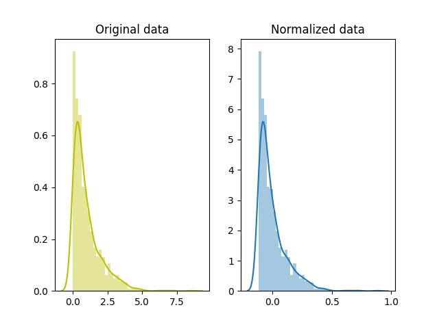
Fig. 6 Normalization
Impact of scaling and shifting random variables (Khan Academy) (6 minutes)
Blended learning: Scaling and normalisation
Read more about scaling and normalisation here (30 minutes).
X_train_glove = np.array(X_train_glove)
X_test_glove = np.array(X_test_glove)

scl = StandardScaler()
X_train_glove_scl = scl.fit_transform(X_train_glove)
X_test_glove_scl = scl.transform(X_test_glove)

y_train_enc = np_utils.to_categorical(y_train)
y_test_enc = np_utils.to_categorical(y_test)
Exercise
Why do we in this case use fit_transform on the train data, and just transform on the test one?
Exercise
Why do we need to scale the data for deep learning?
Let’s give it a try, is really one entry in the data a 300 dimentional vector?
X_train_glove[0]
array([-2.32894737e-02,  3.10668293e-02, -4.39745151e-02, -5.64447939e-02,
        1.02594390e-03,  1.12070525e-02,  3.20235104e-03,  7.77156604e-03,
        2.61046309e-02, -4.52869862e-01, -4.11277637e-04,  6.31472934e-03,
        1.52215995e-02, -1.23579139e-02, -2.16242392e-02,  2.32162979e-02,
       -4.43424024e-02, -3.73341748e-03,  2.22783145e-02,  1.40877916e-02,
        1.95223875e-02,  2.82965936e-02,  4.11917940e-02,  3.25049497e-02,
       -3.15855332e-02,  2.13159509e-02,  7.44692143e-03,  1.43622817e-03,
        3.66777889e-02,  2.16975231e-02,  3.37503478e-02,  6.12806417e-02,
       -3.37418206e-02,  4.43321886e-03, -2.50328988e-01,  5.24989665e-02,
       -4.48994078e-02,  1.51936822e-02, -3.56097259e-02,  5.47690243e-02,
       -2.48268750e-02, -5.78602822e-03, -2.56457441e-02, -2.95194350e-02,
        1.33604351e-02,  4.97801453e-02,  5.30099310e-02,  1.33737382e-02,
       -2.12662108e-02,  3.18849273e-02,  1.54437823e-02,  7.23906280e-03,
        1.78525653e-02, -3.21954787e-02, -1.27164163e-02,  4.35023718e-02,
       -5.51021798e-03,  5.87610248e-03,  2.05822475e-03,  3.60975154e-02,
        3.46094072e-02, -1.36471484e-02,  7.25326240e-02,  2.62633171e-02,
       -2.78102467e-04, -6.12288713e-02,  2.73836013e-02,  4.06630039e-02,
        2.48716865e-02,  1.71409454e-02,  3.17198448e-02, -2.50090007e-02,
        4.84977383e-03,  7.07255900e-02,  5.59879001e-03,  1.39085650e-02,
       -1.90250054e-02,  1.02943247e-02, -4.13045734e-02, -5.57916388e-02,
       -2.31829099e-02, -4.50426601e-02,  5.89222200e-02, -2.77780909e-02,
       -6.66003861e-03,  5.11157978e-03,  3.09338840e-03,  3.72455567e-02,
       -2.70911288e-02,  9.61873494e-03,  4.42472706e-03,  6.35673478e-02,
       -3.58307697e-02, -4.89802547e-02, -1.47702394e-03, -2.47533228e-02,
       -8.09888393e-02, -1.15977796e-02,  4.87653241e-02, -1.12257764e-01,
       -1.96868237e-02,  4.07871231e-02, -5.16530126e-02, -5.55814803e-02,
       -2.43531330e-03, -8.12497921e-03,  2.42574383e-02,  2.44612861e-02,
       -8.50794762e-02,  4.00520451e-02, -3.55438553e-02, -3.82371247e-02,
       -2.40447130e-02, -4.06305753e-02, -2.11961772e-02,  5.62526882e-02,
       -2.53995825e-02,  4.45758924e-02,  1.15506537e-02, -4.56452072e-02,
        1.99450012e-02, -7.51915351e-02,  6.62240535e-02,  1.82880778e-02,
       -3.40038096e-04,  2.03797668e-02,  1.19775673e-02,  3.51503752e-02,
        2.16680523e-02,  1.71746742e-02,  5.21519780e-02,  6.38001934e-02,
        3.20830978e-02,  2.48942710e-02, -8.17613583e-03,  3.68397944e-02,
       -8.21215007e-03, -5.26166800e-03,  6.91096531e-03,  1.57503244e-02,
       -9.40139312e-03,  2.46435567e-03, -9.52579826e-03, -1.54498499e-02,
       -1.01902738e-01, -4.87458194e-04,  1.87341031e-02,  3.90754128e-03,
        1.48044731e-02,  2.11387649e-02,  9.60999541e-03, -1.12161099e-03,
       -3.13932658e-03, -7.34202117e-02,  8.19091648e-02, -1.74888745e-02,
        1.03314398e-02, -3.97811867e-02,  1.97458398e-02,  2.63384972e-02,
        1.50753334e-02, -8.03321972e-02, -2.95290332e-02, -3.53005603e-02,
        2.90658865e-02,  3.72234546e-02,  1.19341612e-02,  2.80832220e-02,
        6.01811446e-02,  1.19202295e-02,  3.54915066e-03,  3.24240364e-02,
       -1.06825657e-01,  3.88127839e-04,  4.20327717e-03, -3.37486668e-03,
       -2.91836057e-02,  5.72584048e-02,  6.08320814e-03,  4.61310707e-03,
        4.08669226e-02, -7.09671155e-03,  5.91302142e-02,  2.67652869e-02,
       -2.04260610e-02, -3.78775001e-02,  7.66344145e-02,  2.55392268e-02,
        5.41477613e-02,  3.66090983e-03, -5.87164331e-03,  4.62315045e-02,
        1.66062042e-02,  3.03641874e-02,  1.10087590e-02, -2.91239731e-02,
       -6.49839118e-02, -1.66033804e-02,  3.49712931e-03, -6.31746128e-02,
        2.16965958e-01,  3.01345438e-02,  7.06991330e-02,  1.92122553e-02,
        4.82732318e-02,  3.37176882e-02, -1.00389728e-02, -1.08275819e-03,
       -2.77451742e-02, -1.83033315e-03, -2.00415570e-02, -1.24214292e-02,
        6.32454008e-02,  5.12878038e-03,  4.00201827e-02, -2.05802638e-03,
        2.77434774e-02, -4.43505403e-03, -2.10391052e-04, -2.60170270e-02,
        3.74035910e-02,  4.92131477e-03, -3.15390006e-02,  4.66568768e-03,
        1.83680877e-02, -1.80903282e-02, -4.40934859e-03, -7.00278580e-03,
        1.51425274e-02, -1.86301786e-02,  4.11494710e-02, -2.14782730e-02,
       -9.28951660e-04, -7.16459155e-02,  4.10312563e-02, -1.95521768e-03,
       -2.33021681e-03,  1.08297542e-02, -1.95159577e-02, -4.89295460e-03,
        3.12124155e-02, -2.53360881e-03,  3.55091505e-02,  2.45698523e-02,
       -1.52898744e-01, -6.18621632e-02,  5.06714843e-02,  3.20858248e-02,
       -3.98602709e-03, -2.43617557e-02,  2.57377047e-02, -4.57251929e-02,
       -9.34164785e-03, -7.73427039e-02,  1.02578342e-01,  1.84447393e-02,
       -4.07262985e-03, -2.34674048e-02, -2.68124905e-03,  2.92026065e-03,
       -5.93280606e-03, -7.20642880e-02, -1.93936769e-02,  2.46707699e-03,
        6.85578771e-03, -2.85296992e-04, -5.18337488e-02,  6.10110164e-03,
        1.05954679e-02,  8.88415705e-03,  6.38094265e-03, -1.39176007e-02,
        3.14134266e-03,  2.20535174e-02, -2.66812649e-02,  2.31649298e-02,
       -5.59711337e-01,  1.06887231e-02,  7.14323344e-03, -4.45074076e-03,
       -4.74225245e-02,  2.58071860e-03,  2.32525598e-02,  4.23671827e-02,
       -2.06068270e-02,  5.04491441e-02,  1.84423141e-02,  2.06283039e-05,
       -1.46646611e-02, -2.02254001e-02, -6.08140416e-03, -1.26735009e-02,
       -4.31094901e-04,  2.02291682e-02,  3.83833423e-02,  2.13016500e-03,
        2.24654120e-03, -6.17554523e-02,  6.78942259e-03,  4.26397696e-02])
Indeed it is. We are now ready to feed this data to a machine learning model, which we will do in the tutorial on Deep Learning in NLP. Now let’s finally export this data for later usage. Using Pickle is the fastest way to achieve this.
pickle.dump(X_train_glove_scl, open("../data/X_train_glove_scl.pkl", "wb"))
pickle.dump(y_train_enc, open("../data/y_train_enc.pkl", "wb"))
pickle.dump(X_test_glove_scl, open("../data/X_test_glove_scl.pkl", "wb"))
pickle.dump(y_test, open("../data/y_test.pkl", "wb"))
pickle.dump(y_test_enc, open("../data/y_test_enc.pkl", "wb"))
Blended learning: Python object serialisation
Read about object serialisation in Python in the official Pickle documentation (30 minutes).
Exercise
Try the built-in pandas methods for object serialisation.
Exercise
The creation of custom word embeddings becomes very useful for domain-specific datasets, where a lot of named entity disambiguation is also required. This is very often the case in the medical domain. Use what you have learned here to create your own embeddings on a medical text dataset, for example: https://www.kaggle.com/tboyle10/medicaltranscriptions
spaCy word vectors
We could also use the embeddings available in spacy.
import spacy

nlp = spacy.load("en_core_web_sm")
tokens = nlp("dog cat banana afskfsd")

for token in tokens:
    print(token.text, token.has_vector, token.vector_norm, token.is_oov)
dog True 19.266302 True
cat True 19.220264 True
banana True 17.748499 True
afskfsd True 20.882006 True
Additional information
Read about the state of the art universal word and sentence embeddings here (1 hour).
Let’s have a look at an individual vector:
tokens[0].vector
array([ 0.99822044, -0.8781611 , -0.9599147 , -0.8802022 ,  1.4011143 ,
       -1.4729911 , -1.4483004 ,  2.3529506 ,  1.4696705 ,  4.1085796 ,
        4.661976  ,  2.9604769 ,  4.635996  , -0.84563375,  0.9116936 ,
       -1.1318729 , -0.92072326,  1.4788682 , -1.4155934 , -2.4691365 ,
       -2.422693  ,  0.87474394, -0.7867575 , -1.8145221 ,  0.7019544 ,
       -1.6173346 , -1.8799448 , -4.580726  ,  1.8491042 , -0.32686716,
        4.730577  ,  0.57223386,  0.7283193 , -0.3618081 , -3.2380333 ,
       -0.6483809 ,  3.613314  ,  0.42308074, -0.49508172,  0.74843705,
        3.9148026 ,  2.307486  ,  0.8387308 , -1.3754001 , -1.1304648 ,
        2.155499  , -1.6760478 , -1.2141752 , -1.2715306 , -1.6553345 ,
       -0.16264206, -1.3702772 , -1.4764215 , -0.7934667 , -1.8332126 ,
        0.7584114 ,  5.2410417 , -0.38271964,  0.6616207 , -1.6419213 ,
        1.3823496 , -0.98040056, -0.2352474 , -0.4358213 ,  0.9533407 ,
       -1.0267448 , -1.1989149 ,  0.44146824, -1.9613253 ,  0.13480479,
       -1.6117922 ,  1.7746817 ,  0.45083126,  1.5055051 , -3.2233422 ,
       -0.6783832 , -1.4262296 , -1.3069394 , -0.26983237,  0.42622554,
        4.113386  , -2.8683515 , -1.6826023 , -1.4485264 ,  0.9647131 ,
        2.2337825 , -0.9116962 , -1.5483243 ,  1.0004147 , -1.803612  ,
       -2.236876  ,  0.6904143 , -2.5448341 ,  2.2533112 , -0.562313  ,
        3.0456731 ], dtype=float32)
We can also compute the similarity between those vectors.
print(tokens[0].similarity(tokens[1]))
0.4805915
Additional information

Word embeddings playground from the University of Turku: http://bionlp-www.utu.fi/wv_demo/
Portfolio Projects
Portfolio Project

Custom word embeddings can be extremely useful when applied to specific domains. In most other cases the pre-trained embeddings, such as the ones obtained from the gensim library can be good enough.
One of the domains which is very specialised, and where information retrieval and abbreviation disambiguation is an issue is healthcare. For this project go and download the medical transcription data from Kaggle and use that to create word embeddings.
Portfolio Project
By using functions such as most_similar we can easily debug a word embeddings model. Still, such work requires programming skills, and often times the data scientist might not be the most useful person to debug this information (think about the first portfolio project here - the medical dataset) - it might require more domain knowledge.
In order to get around this problem, and make the embeddings accessible to a non-technical user, you can create a graphical interface (see diagram below).

Glossary
- GloVe
Global Vectors for Word Representation