3: Supervised Learning
Introduction
Now that we have processed and prepared our data for machine learning we can go ahead and start training a model. This is how we know how good our processing was!
One of the most important libraries that we will use here is scikit-learn, which as you have seen in previous sections is the most popular machine learning libary for Python, and also has some handy text processing functionalities that we will use.
import pandas as pd
from sklearn.preprocessing import LabelEncoder
from sklearn.feature_extraction.text import CountVectorizer, TfidfVectorizer
from sklearn.ensemble import RandomForestClassifier
from sklearn.svm import SVC
from sklearn.model_selection import train_test_split
from sklearn import metrics
![]()
Blended learning: NLP in scikit-learn
At this point you must be very familliar with scikit-learn. It is the workhorse of machine learning in Python, and one of the best maintained and documented open source libraries. Thus it is not surprising that the libary has some additional functionality for working with text data in machine learning. You can go through the official tutorial here to learn more (1 hour).
First we should load the data we processed before. One new thing that we do here is to transform the label as well into a format that is readable by our ML libaries.
reviews_data = pd.read_csv("../data/reviews_data.csv")
reviews_data = reviews_data[["overall", "text_processed"]]
reviews_data = reviews_data.dropna()
reviews_data.sample(10)
| overall | text_processed | |
|---|---|---|
| 2144 | 5.0 | anyon think problem lint look pictur my hous y... |
| 1200 | 3.0 | at first contrapt littl confus i read direct t... |
| 1986 | 5.0 | we foot solid dryer vent pipe end go floor fle... |
| 1902 | 3.0 | first thing first work kit great consist price... |
| 2185 | 5.0 | great |
| 409 | 5.0 | the lint eater amaz we recent bought hous buil... |
| 972 | 3.0 | first thing first work kit great consist price... |
| 1295 | 5.0 | i bought last octob final got around clean dry... |
| 1301 | 4.0 | great product need includ rod kit i buy second... |
| 880 | 3.0 | at first contrapt littl confus i read direct t... |
Exercise
If you look closely at the data you can see that theere are quite a few duplicates in it. As an exercise your job is to check out what options are available for de-duplicating text data.
Of course, there are two types of duplicates - those which are 100% match, and partial ones. Bonus points for finding and implementing a solution for partial matches.
Bag of Words (BoW)
While we have done most of the text processing in the previous chapters (i.e. lemmatization, word embeddings), here we still have a few similar steps we need to do.
The simpler and older (and arguably less accurate) older alternatives to word embeddings is the creation of BoW and TF-IDF.
Bag of Words (7 minutes)

The Bag-of-words is the most basic representation of text data in a tabular format. Here for every text entry we have a row of length n which is the number of unique words in the whole document, and each column corresponds to the number of occurrences of that word in this document.
TF-IDF has a similar approach but takes into account how “important” that word is, and gives it aditional weight. The importance in this case is defined by a word being rare in a document, but common in between.
Additional information: TF-IDF in the wild
If you want to get a deeper understanding on how TF-IDF can be used in the real world, have a look at this article.
Additional information: Manual Annotation and Labeling

You might happen to hear the expression “data is the new oil” thrown around in the community. This statement is mostly true - data is extremely valuable. But it fails to mention exactly what type of data is so valuable - labeled data. This type (different from unsupervised learning approaches) of data is extremely hard to get to, since it often requires manual work by an annotator.
Data annotation can be an extremely tedius task, and the tools that support it need to be very well designed. One such tool used in NLP is called Prodigy. In the above video you can find more information about it.
Another similar tool (but non-commercial) is Snorkel.
An overview on what we are trying to achieve is available on Supervised NLP Overview.
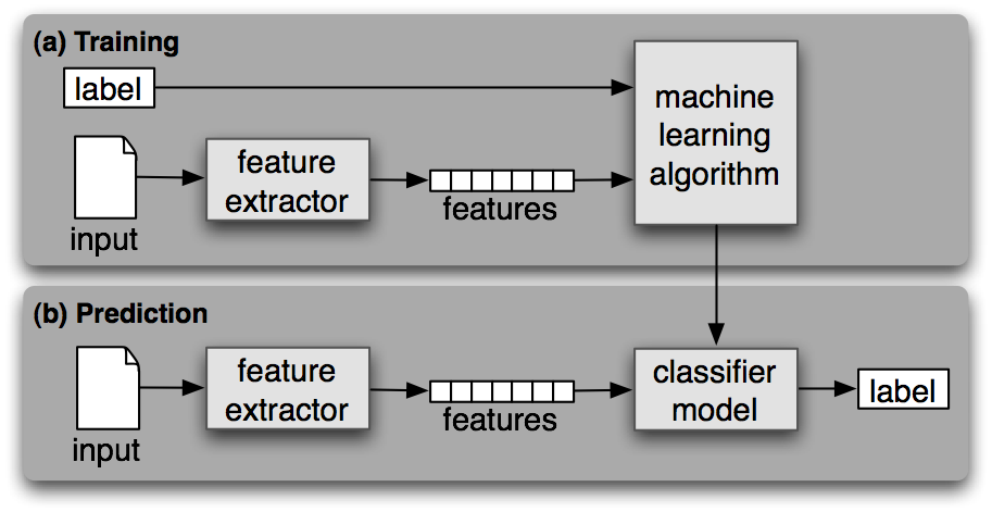
Fig. 7 Supervised NLP Overview
corpus = reviews_data["text_processed"]
y = reviews_data["overall"]
vectorizer_bow = CountVectorizer()
vectorizer_tfidf = TfidfVectorizer()
X_bow = vectorizer_bow.fit_transform(corpus)
X_tfidf = vectorizer_tfidf.fit_transform(corpus)
Now let’s have a look at the datatype of the resulting object:
type(X_bow)
scipy.sparse.csr.csr_matrix
Perhaps you were expecting a dataframe, but we got this instead. The keyword in the description is sparce. And sparce datasets are those which contain many constant values, in our case we will have lots of zeroes, since there will be a lot of words which are present in one document but not others. The memory footprint of sparse dataframes is optimised for such use cases, and they take less space than a normal dataframe.
Now let’s create a Random Forest model and see which preprocessing step is better?
Blended learning: Sparce Matrices
Learn more about sparse matrices and how they can be used in machine learning on Machine Learning Mastery (1 hour).
What is TF-IDF? (10 minutes)

X_train, X_test, y_train, y_test = train_test_split(X_bow, y, test_size=0.33, random_state=42)
clf_rf_bow = RandomForestClassifier()
clf_rf_bow.fit(X_train, y_train)
preds_rf_bow = clf_rf_bow.predict(X_test)

X_train, X_test, y_train, y_test = train_test_split(X_tfidf, y, test_size=0.33, random_state=42)
clf_rf_tfidf = RandomForestClassifier()
clf_rf_tfidf.fit(X_train, y_train)
preds_rf_tfidf = clf_rf_tfidf.predict(X_test)
print('Accuracy of BOW is {}'.format(metrics.accuracy_score(y_test, preds_rf_bow)))
Accuracy of BOW is 0.9906666666666667
print('Accuracy of TF-IDF is {}'.format(metrics.accuracy_score(y_test, preds_rf_tfidf)))
Accuracy of TF-IDF is 0.9893333333333333
As a result you can see that TF-IDF is marginally better for this use case, but not significantly different.
Another thing that we can do is try to use a different model. One which is generally effective in text classification tasks are Support Vector Machines. Let’s try, this time just with tf-idf:
clf_svc = SVC()
clf_svc.fit(X_train, y_train)
preds_svc = clf_svc.predict(X_test)
print('Accuracy of SVC is {}'.format(metrics.accuracy_score(y_test, preds_svc)))
Accuracy of SVC is 0.9893333333333333
Roughly the same, but it was worth a try!
Exercise
Using the same dataset, try setting up fasttext’s classifier, and compare it’s performance.

Additional information: Sentiment Classification
Recognizing the sentiment of text can be very valuable for quite a few different business applications. For example, we would be interested in knowing what is the sentiment of the user reviews of our products online (i.e. on social media). This can be automated by building sentiment prediction models.

There are quite a few methods to achieve that, and in order to get an understanding you can read the groundbreaking research on the topic by OpenAI.
Sentiment Classification with Naive Bayes (1 hour)
Deep Learning
Large amounts of compute power and an always increasing amount of unstructured data have turned the deep learning field in a revolution in data science. Many of the methods that have since exploded in usefulness and popularity would not be possible earlier because of those constraints.
Additionally, the development of more open and easy to use open-source tools which are suitable for a production envrionment, together with cloud computing, have made deep learning all the more accessible to a larger audience of technical data people.
![]()
One such great example is Keras, which has since been integrated within Tensorflow (in version 2.0). This library allows people with little knowledge in the intricacies of deep learning to build their own first models, and this is why we will focus on it in the current course.
import pickle
from sklearn import metrics
from keras.models import Sequential
from keras.layers.recurrent import LSTM, GRU
from keras.layers.core import Dense, Activation, Dropout
from keras.layers.embeddings import Embedding
from keras.layers.normalization import BatchNormalization
X_train_glove_scl = pickle.load(open("../data/X_train_glove_scl.pkl", "rb"))
y_train_enc = pickle.load(open("../data/y_train_enc.pkl", "rb"))
X_test_glove_scl = pickle.load(open("../data/X_test_glove_scl.pkl", "rb"))
y_test = pickle.load(open("../data/y_test.pkl", "rb"))
y_test_enc = pickle.load(open("../data/y_test_enc.pkl", "rb"))
Blended learning: FastAI
We have been using word embeddings for normal text data, but did you know that you could use the same context for categorical data? An excellent introduction is available on fast.ai (2 hours).
And now to construct our neural network. Here the magic of Keras shines with the high level API, where we need to only know the most important pieces of a neural network:
Getting started with Keras (8 minutes)

model = Sequential()
model.add(Dense(300, input_dim=300, activation="relu"))
model.add(Dropout(0.2))
model.add(BatchNormalization())

model.add(Dense(300, activation="relu"))
model.add(Dropout(0.3))
model.add(BatchNormalization())

model.add(Dense(6))
model.add(Activation("softmax"))

model.compile(loss="binary_crossentropy", optimizer="adam", metrics=["accuracy"])
And in the next step we can proceed to train this neural network on the data.
model.fit(X_train_glove_scl, y=y_train_enc, batch_size=64, epochs=5, verbose=1, validation_data=(X_test_glove_scl, y_test_enc))
Epoch 1/5
24/24 [==============================] - 0s 15ms/step - loss: 0.1634 - accuracy: 0.8393 - val_loss: 0.0463 - val_accuracy: 0.9787
Epoch 2/5
24/24 [==============================] - 0s 4ms/step - loss: 0.0225 - accuracy: 0.9862 - val_loss: 0.0244 - val_accuracy: 0.9840
Epoch 3/5
24/24 [==============================] - 0s 5ms/step - loss: 0.0096 - accuracy: 0.9967 - val_loss: 0.0222 - val_accuracy: 0.9867
Epoch 4/5
24/24 [==============================] - 0s 5ms/step - loss: 0.0063 - accuracy: 0.9961 - val_loss: 0.0205 - val_accuracy: 0.9867
Epoch 5/5
24/24 [==============================] - 0s 5ms/step - loss: 0.0056 - accuracy: 0.9967 - val_loss: 0.0241 - val_accuracy: 0.9867
<tensorflow.python.keras.callbacks.History at 0x7f8f9dd88b00>
And finally, let’s have a look at the performance of the model:
nn_preds = model.predict_classes(X_test_glove_scl)
print('Accuracy of neural network is {}'.format(metrics.accuracy_score(y_test, nn_preds)))
Accuracy of neural network is 0.9867021276595744
Exercise

One of the great tools available in the TensorFlow package is Tensorboard. This allows you to explore interactively the results and parameters of machine learning training and testing. As an exercise, set it up for the current project.
Blended learning: TFhub
We already mentioned TensorFlow before. TFHub is another service related to it which allows the reuse of machine learning models. Have a look at the following tutorial on how to classify text with Keras (2 hours).
Blended learning: CNN
Another type of neural network that you can use for text classification is CNN. Go through this tutorial on how to do that with the official Keras documentation (2 hours).
![]()

Text Classification Using Convolutional Neural Networks (15 minutes)
Exercise
Compare the results of a deep learning algorithm to a state-of-the-art tree-based method, such as xgboost, or catboost.
Exercise
Experiment with the network architecture based on the blended learning. Are there new optimisations that can make the model a bit more accurate?
Exercise
If you had to train and test different neural network architectures and parameters, how would you do it in a productive way? Can you find tools that can help you with that, and how would you achieve it yourself?
Portfolio projects
Portfoio project

Some of the most common users of NLP technology in the real world are news organisations. They face a lot of challenges, especially since the digitialisation has begun. Those challenges also provide them with opportunities to use new technologies.
One of the most useful machine learning applications for news is content categorisation 1. This can help news organisations provide functionality on their website where content is grouped accordingly. Before this job had been done manually, but it can now be automated with ML.
Your project is to download the data from here and create a classifier using what you have learned. Bonus points for attempting a deep learning approach.
Portfolio Project

During this module you have alraedy encountered one common problem that NLP can solve - duplicate detection. You can test your new found NLP skills on the Quora duplicate questions challenge.
Here is the description from the Kaggle website:
The goal of this competition is to predict which of the provided pairs of questions contain two questions with the same meaning. The ground truth is the set of labels that have been supplied by human experts. The ground truth labels are inherently subjective, as the true meaning of sentences can never be known with certainty. Human labeling is also a ‘noisy’ process, and reasonable people will disagree. As a result, the ground truth labels on this dataset should be taken to be ‘informed’ but not 100% accurate, and may include incorrect labeling. We believe the labels, on the whole, to represent a reasonable consensus, but this may often not be true on a case by case basis for individual items in the dataset.
Glossary
- BoW
Bag of Words
- CNN
Convolutional Neural Network
- TF-IDF
term frequency–inverse document frequency
- XGBoost
eXtreme Gradient Boosting